Hubble Diagram
Edwin Hubble examined galaxies outside of the Milky Way. With the limited types of telescopes in the early 20th century, Hubble had to find alternate ways of examining these qualities than what we are used to doing with our naked eye. Now, we have even better telescopes that exceed what Hubble was able to do then. Hubble compared the velocity and distance of galaxies to prove that the Universe was expanding. How did Hubble do this? How accurate was he? Have we gotten better measurments since then? These questions and more are what we will examine today.
Hubble's 1929 paper contains data that, with a little work, we can plot. Astronomers have repeated this exercise with data from larger galaxy surveys and a variety of calibration techniques. Let's do what he did. The first six columns copy the information in table 1 from the paper. The first column is the name of the object. S. Mag and L. Mag refer to the small and large Magellanic clouds. The rest are numbers in the New General Catalog compiled in the 19th century. The objects in this catalog are spectacular! They have been photographed and cataloged many times by professional and amateur astronomers. For example, here is how to see information about NGC598, the fourth object in Table 1. The rest of the columns are described in the paper. Note that in the last column, all of the values are negative. The style in tables is to imply the repetition of a prefix of the entry in the first row. When signs change, as in the velocity column, it is made explicit. We are interested in r, the distance (given in units of mega-parsecs) and velocity (given in units of kilometers per second.) We plot those in the chart. Compare this chart to the version in the paper. We also fit these points two ways, with and without forcing the line through the origin. How do these slopes compare with values given in the paper? A way to quantify how well data are correlated is the r-squared, which for linear regression is the correlation coefficient squared. An absolute value of 0.0 means the data are not correlated at all; 1.0 means they are perfectly correlated. Compare the r-squared value for this fit with the examples. Note the value for Hubble's data to compare with values in the next exercise. The slope of this line is now called the "Hubble Constant", H. Notice its odd units: kilometers per second per megaparsec. This turns out to be in units of inverse time, and 1/H is known as the "Hubble Time." Calculate this time in years, using the fact that one parsec is 3 x 10^16 meters, for the slopes you obtain. What is that time in years? (Note: the tab "Hubble Time" works this out.) In the early 1930s, the accepted age of the earth, based on ratios of isotopes found in geological samples, was 2 to 3 billion years. Based on our understanding of how stars are born and burn, astronomers generally agreed that the age of the stars are an order of magnitude larger. Is there a problem here? In 1932, a prominent cosmologist Willem DeSitter wrote "I am afraid all we can do is to accept the paradox and try to accommodate ourselves to it, as we have done to so many paradoxes lately in modern physical theories." (Cosmology and Controversy, Helge Kragh, 1999, p 74) In the 1929 paper, Hubble points out the importance of knowing the correct absolute magnitude of objects to use when converting from apparent magnitude to distance: "Distances of extra-galactic nebulae depend ultimately upon the application of absolute-luminosity criteria to involved stars whose types can be recognized." The last column in the table calculates the distance based on the apparent and absolute magnitudes from other columns. This is the equation we will use in the next exercise.
Distance
How do we measure distance? Our eyes use depth perception and brightness to guage distance. Examples are rulers, meter sticks, and micrometers. On an astronomical level we do the same thing. Astronomers use crazy units. They have come up with new ways to measure distances so that the numbers are easier to wrap our head around. For example, I could tell you the Sun is 149.60 X 10^9 meters away. This is a hard number to imagine so astronomers came up with a new unit, the Astronomical Unit (clever name). The Astronomical Unit (AU) is the mean distance from the Earth to the Sun. So if I say that Jupiter is about 5.2 AU from the Sun, one can imagine that Jupiter is roughly five times farther away from the Sun than Earth. Five is a much easier number to imagine than 149.6 X 10^9.
So how did Hubble measure distances? With a really big ruler!?! Not exactly. With a yard stick. But really, Hubble had to look at other characteritics of the star that were dependent on distance. In other words, as distance increases what other observable qualities about the star change? Current astronomers look at many different things including brightness, angular size, lumpiness, and the appearence of objects in front of and behind the galaxies. With Hubble's limited technology, he chose brightness. As objects get closer they get brighter, and as they get farther away they get dimmer. Distance and brightness are directly related by the familiar (1/r2) law. However, brightness seems like a fairly qualitative measurement. How exactly did Hubble (and many astronomers since then) measure brightness. Below is a night image of the city of Honolulu. There are different colored lights, different brightness of lights, but our eyes can still pretty much measure the depth and distance of objects. If something is bright does that mean its closer? If not, then how do we differentiate between bright distant objects and dim near objects? In order to do this we need some sort way of telling the "absolute brightness" of each object. If we know what the intrinsic brightness of the light bulb is, and we know what it looks like, we can determine the distance.

Brightness and Magnitude
Astronomers keep track of the brightness of objects and their distance by giving them a value we call magnitude. The equation defining magnitude is,
m = -2.5log(# of photons/sec)
Note the negative sign, so magnitude is on an inverse scale. This means that a really bright star might have a magnitude of -10, while a really dim star might have a magnitude of 25. There are also two different types of magnitude. There is apparent magnitude (m), and absolute magnitude (M). Apparent magnitude corresponds to the magnitude (brightness) seen from Earth. Absolute magnitude is the magnitude the object would have if it were 10 parsecs away. A parsec is another measurement of distance made up by astronomers. One parsec is approximately 31 trillion kilometers away. The derivation of the parsec is an interesting one, but not useful in our activity. Basically, the absolute magnitude is a way of comparing many objects' brightnesses at the same distance. In addition to being on an inverse scale, magnitude is also on a log scale. Each step is 100.2 difference in brightness. By knowing absolute and apparent magnitude, we can determine the distance of a galaxy.
Originally magnitude was measured fairly subjectively. As technology increased we began to take spectra of stars, galaxies, and and other celestial objects. Through the Sloan Digital Sky Survey (SDSS), there are known spectra for thousands of galaxies. Once we have the apparent magnitude from the spectrum and define an absolute magnitude to the object, we can use the 1/r2 law to calculate d. The equation is
d=10^ (.2(m-M)+5)
In case you need to dust up on your algebra skills or just like seeing mathematical derivations, click here for the full explanation on this.
Math for Magnitude to Distance Calculation
Below is the link to freely navigate objects in the sky from SDSS.
- Directions for working the navigation tool on SDSS - After opening the navigation tool there are options on the left hand side to view different characteristics. If you click on "objects with spectra," SDSS will automatically outline objects with known spectral data with a red box. Use the navigation keys to find an object with a red box around it and click on it. On the right hand side you have the option to get a "quick look" at the object. Click the "quick look" button and a new window should open. On the left there is a list of magnitudes, and on the right there is the actual spectral graph. For our activity we will use the "r" magnitude, measured through teh "r" filter on the telescope. Some fun activities to do using the Navigation tool on Sky Server could be finding galaxies with specific "r" values or searching for anything fun through pictures of hte sky.
Velocity
How do we measure the velocity of a star or galaxy? This is where it starts to get a little tricky. Many of you are aware of or have experienced the Doppler Effect. In general. the doppler effect occurs when an object is moving in relation to you and you hear the sound it makes change while its position changes. This happens because the sound wavelenghts are being stretched or contracted. Since we are examining light wavelengths, a similar phenomenon happens when looking at the light from objects in the universe. We call this redshift. Below is a great youtube video explaining redshift.
If you go back and use the navigation tool from SDSS and go through the same steps you will see a value for redshift (z) on the right side.
Plotting Distance vs Velocity
We've now looked at magnitude and redshift and see that they are related to distance and velocity. Lets try plotting a large amount of galaxies in the universe and see what happens. As a side note, when Hubble compared distance and velocity of galaxies, he saw a relationship. Lets try it out and see. Open up the excel document and click on the first tab labelled "All Galaxies." This tab holds the first 10,000 galaxies with spectra that SDSS has. The first four columns are data from SDSS. The other two columns of data are the calculated distance and velocity. Graph distance vs. velocity and lets see what we come up with. Does it look like what Hubble predicted? Do you see a linear relationship? Why or why not?
Click on the second tab of the excel sheet labelled "z>.25" This tab has data from the first 10,000 galaxies with sepctra like the one before, but this one only has galaxies with a redshift value over .25. Lets graph distance vs velocity and see what it looks like. Can you do a linear fit to it? What has changed since the first graph?
Velocity Dispersion
We now see that comparing solely distance and magnitude does not work. We need to be careful to compare similar galaxies with similar intrinsic qualities. When comparing galaxies it is helpful to use an analogy about lightbulbs. There are many different types of lightbulbs and many of them have different wattages. If one were in a dark room surrounded by lightbulbs of all different wattages it might be hard to tell which ones were closer, and which ones are further away. For example, a 30 watt lightbulb that is only one meter away might look brighter than a 120 watt lightbulb that is 30 meters away.
Thus, comparing their distances and velocities from our viewpoint might be hard if we don't know which one is intrinsically brighter. One way that astronomers go about doing this when observing galaxies is to look at something call the velocity dispersion. A velocity dispersion is a measure of velocities in a specific galaxy. Since galaxies are spinning and they're made up of spinning stars there are different red and blue shifts visible on either side of the center. The velocity dispersion is a number that pulls all the velocities in different directions together and gives something comparable to the total spin of a galaxy. Although it is not that simple. Because of the mass present, larger galaxies spin faster and smaller galaxies spin slower. So in our activity we are using velocity dispersion as a type of mass measurement. Velocity dispersion is measured in km/s. By zooming in on a specific velocity dispersion we can compare similar galaxies and are no longer comparing things of different watts as in our example. So picking a velocity dispersion is similar to picking a specific wattage to examine. Below is a histogram of all possible velocity dispersions. A histogram graphs a number across the bottom (in our case the different possible velocity dispersions), and on the vertical scale it shows the number of time that velocity dispersion occurs in our data.

Hopefully you can see by the above graph that most of the velocity dispersions occur around 160 km/s. Thus SDSS has more data of galaxies with velocity dispersions of 160 km/s than a higher or lower velocity dispersion. However, it is important to note that we have more accurate data for higher velocity dispersions. This is because velocity dispersions is measured from the spectrum of a galaxy. We see better and more clear spectra from larger galaxies because we can get more light from them. Thus the higher velocity dispersions are more accurate even though there are less of them.
Excel Sheet Activity Directions
- First make sure you are on the first tab of the spreadsheet labeled, "Veldisp 140, (180,0)." The reason the spreadsheet is named this is correesponding to the specific velocity dispersion that has been given (140 km/s), and the RA and Dec position we are examining in the sky. For a quick lesson on RA and Dec click HERE. SDSS has data only in certain areas of RA and dec. Directions 2 and 3 show an image of the footprint of what SDSS has mapped. So for our first tab, we have picked an area with a radius of 3 degrees where RA = 180 and Dec = 0.
- The first four columns on the spreadsheet are raw data from the SDSS database. The first column is the red magnitude (apparent magnitude), the second column is the redshift, and the third and fourth columns are RA and Dec.
- Under the calculated data we have changed the magnitude to a distance and the redshift to a velocity. There are two separate steps in order to do this.
- To change magnitude into distance we need an equation. The equation uses apparent magnitude and absolute magnitude. We got the apparent magnitude from the spectrum of the galaxy. When we picked a velocity dispersion we made the assumption that for galaxies with a specific velocity dispersion they have a similar (if not the same) absolute magnitude. We will not go into the derivation but there is a relationship between velocity dispersion and magnitude. For our purposes we just pick a reasonable absolute magnitude and be sure to use it the entire time. On the spreadsheet we have absolute magnitude set at -10. The equation relating magnitude to distance is, d= 10^(.2*(m-M)+5). Where d is distance, m is apparent magnitude, M is absolute magnitude and d comes out in parsecs. Since we want our answer in units of MPc we divide the entire thing by 1,000,000. This is what you see in column F.
- To change redshift to velocity we also need an equation. Since redshift is a percentage of the speed of light we multiply c*z, where c is the speed of light. c=3*10^8. Thus, v=(c*z)/1000. We divide by 1000 because the speed of light comes in m/s and we want km/s. This is what you see in column G.
- Now you can go ahead and graph distance vs. velocity in excel. Do a linear fit (making sure to set the intercept to 0 since we want that sort of fit), and record the slope.
- In the next tab you can do the same activity but looking at a different RA and dec. This way you can see if the universe is expanding with the same approximate rate in another part of the sky. In the tab labelled "Veldisp 140, (210,0)," the equations for the distance and velocity are not already programmed in. You can play around and model them after the first tab. We are looking at the same types of stars (constant velocity dispersion) but in a different part of the sky. Are they moving away from us at the same rate? Depending on your answer what does this mean?
- The third tab labeled "Veldisp 210, (180,0)," is the same idea but you are back to looking at the original part of the sky but examining galaxies with a different velocity dispersion. Will the expansion rate be the same? Why don't you find out!
- The excel sheet has three extra tabs where you can fill in the colored cells to reflect the data YOU choose to look at. Be sure to change your tab names so you can remember what data you used where.
Additional Data Analysis
Now that you have analyzed three different graphs lets brainstorm some other ideas we can do with the data. The two main variables we can switch around are the velocity dispersion and the place in the sky. Do all objects with a certain velocity dispersion have similar expansion rates? Or does it depend on the location in the sky? What about galaxies in the same area of the sky but with different velocity dispersions? We'll show you how to pull the data off the database yourself and then you can design your own questions and look into the answers. The search database we use for getting this data is SQL. The link is below
Directions for Using SQL Search
- Open up SQL and delete the preset things typed into the white box.
- SQL works on a three definition search. Type each word in a different line, Select, From, Where
- Select is the function that tells SQL what data you want out of it. Since we have been looking at magnitude, redshift, RA, and Dec, these are what you want to specify. The Select line should look like step four.
- Select Top 1000 mag_1, z, ra, dec
- The top 1000 function allows us to put a maximum number of data points we want. Mag_1 corresponds to the red magnitude we have been using. Z is the symbol for redshift, and RA and dec are what they sound like.
- From is the function that tells SQL where to get our data from. We're looking for objects with spectrum and objects that are near a certain position in the sky. The From line should look like step seven separated by an enter.
- From specobj as G, [ press enter] dbo.fgetnearbyobjeq(180,0,60) as N
- the (180,0,60) corresponds to (RA, Dec, radial arcmin to look around). In our example we use an RA of 180, a dec of 0, and you should almost always use a radial arcmin of 60.
- The Where line tells SQL what limitations we want on our data. Line 10 shows what the where line should look like.
- Where (G.bestobjid = N.objid) and (veldisp between 200 and 220) and (veldisperr<40)
- The "veldisp between" tells SQL where we want to limit our velocity dispersion. Veldisperr is the error on the velocity dispersion and we want to keep that reasonably low.
- SQL does not care about capital letters and lower case letters
- Before you click submit, choose an output format of "CSV." This should pull your data up in an excel file so it is easy to copy and paste into your excel sheet. Below is a screen shot image of our example.
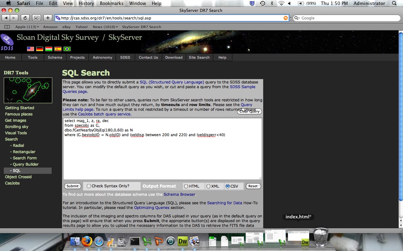
See what data you can pull off the database using SQL and examine the ways that the hubble diagram changes as we change the velocity dispersion and the position in the sky.